基本操作
安装
1
|
pip install numpy opencv-python pillow matplotlib
|
numpy 的一些例子
- Creating NumPy Arrays
 1
 2
 3
 4
 5
 6
 7
 8
 9
10
11
12
13
14
15
16
17
18
19
20
21
22
23
24
25
26
27
28
29
30
31
32
33
|
import numpy as np

# Create an array from a list
arr1 = np.array([1, 2, 3, 4])
print(arr1)

# Create a 2D array (Matrix)
arr2 = np.array([[1, 2, 3], [4, 5, 6]])
print(arr2)

# Create an array of zeros
arr3 = np.zeros((3, 3))  # Shape (3,3)
print(arr3)

# Create an array of ones
arr4 = np.ones((2, 4))  # Shape (2,4)
print(arr4)

# Create an array with random values
arr5 = np.random.rand(3, 3)  # Uniform distribution
print(arr5)

# Create an array with values from a normal distribution
arr6 = np.random.randn(3, 3)  # Standard normal distribution
print(arr6)

# Create an array with a range of numbers
arr7 = np.arange(10, 50, 5)  # Start from 10, step by 5
print(arr7)

# Create a linearly spaced array
arr8 = np.linspace(0, 10, 5)  # 5 values between 0 and 10
print(arr8)
|
- Checking Properties of an Array
1
2
3
4
5
6
|
arr = np.random.rand(3, 4)

print("Shape:", arr.shape)  # Get the shape
print("Size:", arr.size)  # Get the total number of elements
print("Data type:", arr.dtype)  # Get the data type
print("Number of dimensions:", arr.ndim)  # Get the number of dimensions
|
- Reshaping and Flattening
 1
 2
 3
 4
 5
 6
 7
 8
 9
10
|
arr = np.arange(1, 13).reshape(3, 4)  # Reshape to (3,4)
print(arr)

# Flatten to 1D
arr_flat = arr.flatten()
print(arr_flat)

# Transpose the array
arr_T = arr.T  # Swaps rows and columns
print(arr_T)
|
- Indexing and Slicing
 1
 2
 3
 4
 5
 6
 7
 8
 9
10
11
12
13
|
arr = np.array([[10, 20, 30], [40, 50, 60], [70, 80, 90]])

# Access a single element
print(arr[1, 2])  # Element at row index 1, column index 2 (60)

# Get a row
print(arr[0, :])  # First row

# Get a column
print(arr[:, 1])  # Second column

# Slice a submatrix
print(arr[0:2, 1:])  # Top-right 2x2 submatrix
|
- Mathematical Operations
 1
 2
 3
 4
 5
 6
 7
 8
 9
10
11
12
13
14
15
16
17
|
a = np.array([1, 2, 3])
b = np.array([4, 5, 6])

# Element-wise operations
print(a + b)  # [5, 7, 9]
print(a - b)  # [-3, -3, -3]
print(a * b)  # [4, 10, 18]
print(a / b)  # [0.25, 0.4, 0.5]

# Square root
print(np.sqrt(a))

# Exponentiation
print(np.exp(a))

# Logarithm
print(np.log(a))
|
- Matrix Multiplication
 1
 2
 3
 4
 5
 6
 7
 8
 9
10
11
12
13
|
A = np.array([[1, 2], [3, 4]])
B = np.array([[5, 6], [7, 8]])

# Element-wise multiplication
print(A * B)

# Matrix multiplication
C = np.matmul(A, B)
print(C)

# Alternative matrix multiplication
C_alt = A @ B
print(C_alt)
|
- Statistical Operations
1
2
3
4
5
6
7
8
|
arr = np.random.rand(3, 3)

print("Mean:", np.mean(arr))  # Average value
print("Sum:", np.sum(arr))  # Sum of all elements
print("Min:", np.min(arr))  # Minimum value
print("Max:", np.max(arr))  # Maximum value
print("Standard Deviation:", np.std(arr))  # Standard deviation
print("Variance:", np.var(arr))  # Variance
|
- Boolean Masking
1
2
3
4
5
6
7
8
|
arr = np.array([10, 20, 30, 40, 50])

# Get elements greater than 25
print(arr[arr > 25])  # [30, 40, 50]

# Replace values conditionally
arr[arr > 25] = 100
print(arr)  # [10, 20, 100, 100, 100]
|
- Stacking and Concatenation
1
2
3
4
5
6
7
8
|
a = np.array([[1, 2], [3, 4]])
b = np.array([[5, 6], [7, 8]])

# Concatenate along rows
print(np.hstack((a, b)))  # Horizontal stack

# Concatenate along columns
print(np.vstack((a, b)))  # Vertical stack
|
- Saving and Loading Data
1
2
3
4
5
6
7
8
|
arr = np.random.rand(3, 3)

# Save to a .npy file
np.save("array.npy", arr)

# Load from a .npy file
loaded_arr = np.load("array.npy")
print(loaded_arr)
|
tensor 的一些例子
- Creating Tensors
 1
 2
 3
 4
 5
 6
 7
 8
 9
10
11
12
13
14
15
16
17
18
19
20
21
|
import torch

# Create a tensor from a list
t1 = torch.tensor([[1, 2], [3, 4]])
print(t1)

# Create a tensor of zeros
t2 = torch.zeros(3, 3)  # Shape (3,3)
print(t2)

# Create a tensor of ones
t3 = torch.ones(2, 3)
print(t3)

# Create a tensor with random values
t4 = torch.rand(2, 2)
print(t4)

# Create a tensor with specific values and data type
t5 = torch.tensor([1.5, 2.3, 3.1], dtype=torch.float32)
print(t5)
|
- Checking Tensor Properties
1
2
3
4
5
|
t = torch.rand(3, 3)

print("Shape:", t.shape)  # Get shape
print("Data type:", t.dtype)  # Get data type
print("Device:", t.device)  # Check device (CPU/GPU)
|
- Reshaping and Manipulating Tensors
 1
 2
 3
 4
 5
 6
 7
 8
 9
10
11
12
13
14
|
t = torch.arange(1, 7).reshape(2, 3)  # Create tensor [1,2,3,4,5,6] and reshape
print(t)

# Transpose
t_transposed = t.T  # Swap rows and columns
print(t_transposed)

# Flatten
t_flattened = t.view(-1)  # Convert to 1D tensor
print(t_flattened)

# Expand dimensions
t_unsqueeze = t.unsqueeze(0)  # Adds a new dimension
print(t_unsqueeze.shape)  # Shape: (1, 2, 3)
|
- Basic Math Operations
 1
 2
 3
 4
 5
 6
 7
 8
 9
10
11
12
13
14
15
16
17
18
|
a = torch.tensor([1, 2, 3])
b = torch.tensor([4, 5, 6])

# Element-wise operations
print(a + b)  # [5, 7, 9]
print(a - b)  # [-3, -3, -3]
print(a * b)  # [4, 10, 18]
print(a / b)  # [0.25, 0.4, 0.5]

# Matrix multiplication
A = torch.rand(2, 3)
B = torch.rand(3, 2)
C = torch.matmul(A, B)  # Matrix multiplication
print(C.shape)  # (2,2)

# Alternative matrix multiplication
C_alt = A @ B
print(C_alt.shape)
|
- Tensor Indexing & Slicing
 1
 2
 3
 4
 5
 6
 7
 8
 9
10
11
12
13
14
|
t = torch.arange(1, 10).reshape(3, 3)
print(t)

# Get a single value
print(t[0, 0])  # First element

# Get a row
print(t[1, :])  # Second row

# Get a column
print(t[:, 2])  # Third column

# Get a submatrix
print(t[0:2, 1:])  # Top-right 2x2 submatrix
|
- Moving Tensors to GPU
1
2
3
4
5
6
|
if torch.cuda.is_available():
    device = torch.device("cuda")  # Get GPU device
    t_gpu = t.to(device)  # Move tensor to GPU
    print(t_gpu)
else:
    print("CUDA not available")
|
- Creating Tensors for Deep Learning
1
2
3
|
# Requires gradient for backpropagation
x = torch.tensor([2.0, 3.0], requires_grad=True)
print(x)
|
- Converting Between NumPy & Tensor
1
2
3
4
5
6
7
8
|
import numpy as np

# Convert NumPy array to Tensor
np_array = np.array([1, 2, 3])
torch_tensor = torch.tensor(np_array)

# Convert Tensor to NumPy array
back_to_numpy = torch_tensor.numpy()
|
| Package |
Purpose |
| numpy |
Used for handling image data as arrays. |
| opencv-python (cv2) |
Used for image processing and manipulation. |
| pillow (PIL.Image) |
Used for opening, editing, and saving images. |
| matplotlib |
Used for visualizing images and plotting data. |
一个例子
 1
 2
 3
 4
 5
 6
 7
 8
 9
10
11
12
13
14
15
16
17
18
19
20
21
22
23
24
25
26
27
28
29
30
31
32
33
34
35
36
37
38
39
40
41
|
import numpy as np
import cv2
from PIL import Image
import matplotlib.pyplot as plt

# Load the image
image_path = "/data/python/peace.jpg"
image = Image.open(image_path).convert("RGB")  # Ensure it's RGB
image_np = np.array(image)  # Convert to NumPy array

# Split RGB channels
R, G, B = image_np[:, :, 0], image_np[:, :, 1], image_np[:, :, 2]

# Create Red, Green, and Blue channel images
red_image = np.zeros_like(image_np)
green_image = np.zeros_like(image_np)
blue_image = np.zeros_like(image_np)

red_image[:, :, 0] = R  # Red channel
green_image[:, :, 1] = G  # Green channel
blue_image[:, :, 2] = B  # Blue channel

# Convert back to PIL images
red_pil = Image.fromarray(red_image)
green_pil = Image.fromarray(green_image)
blue_pil = Image.fromarray(blue_image)

# Concatenate images horizontally
final_image = np.hstack([np.array(image), red_image, green_image, blue_image])
final_pil = Image.fromarray(final_image)

# Show the final concatenated image
plt.figure(figsize=(15, 5))
plt.imshow(final_image)
plt.axis("off")
plt.show()

# Save the final image
final_pil.save("/data/python/rgb_channels_combined.png")

print("Saved the concatenated RGB channel image as 'rgb_channels_combined.png'")
|
原图

转换后的 RGB 拼接的结果

深入
启动
1
|
jupyter notebook --ip=0.0.0.0 --allow-root
|
Torchvision 读取和训练
安装
1
2
3
4
5
|
pip install torchvision
pip install pillow
pip install torch torchvision matplotlib
pip install transformers
pip install opencv-python
|
相关 API
介绍
- torchvision.datasets这个包本身并不包含数据集的文件本身
- 它的工作方式是先从网络上把数据集下载到用户指定目录
- 然后再用它的加载器把数据集加载到内存中。最后,把这个加载后的数据集作为对象返回给用户
MNIST
例子
 1
 2
 3
 4
 5
 6
 7
 8
 9
10
11
12
13
14
15
16
17
18
19
20
21
22
23
|
import torch
import torch.nn as nn
import torch.optim as optim
import torchvision
import torchvision.transforms as transforms
import matplotlib.pyplot as plt

# Define transformations (convert images to tensors and normalize)
transform = transforms.Compose([
    transforms.ToTensor(),  # Convert to Tensor
    transforms.Normalize((0.5,), (0.5,))  # Normalize the data
])

# Download and load the training dataset
train_dataset = torchvision.datasets.MNIST(root='./data', train=True, transform=transform, download=True)
train_loader = torch.utils.data.DataLoader(train_dataset, batch_size=64, shuffle=True)

# Download and load the test dataset
test_dataset = torchvision.datasets.MNIST(root='./data', train=False, transform=transform, download=True)
test_loader = torch.utils.data.DataLoader(test_dataset, batch_size=64, shuffle=False)

# Check dataset size
print(f"Training samples: {len(train_dataset)}, Test samples: {len(test_dataset)}")
|
定义
 1
 2
 3
 4
 5
 6
 7
 8
 9
10
11
12
13
14
15
16
17
18
19
20
21
|
class SimpleCNN(nn.Module):
    def __init__(self):
        super(SimpleCNN, self).__init__()
        self.conv1 = nn.Conv2d(1, 16, kernel_size=3, padding=1)  # Conv layer 1
        self.conv2 = nn.Conv2d(16, 32, kernel_size=3, padding=1)  # Conv layer 2
        self.fc1 = nn.Linear(32 * 7 * 7, 128)  # Fully connected layer 1
        self.fc2 = nn.Linear(128, 10)  # Fully connected layer 2 (output)

    def forward(self, x):
        x = torch.relu(self.conv1(x))
        x = torch.max_pool2d(x, 2)  # 28x28 -> 14x14
        x = torch.relu(self.conv2(x))
        x = torch.max_pool2d(x, 2)  # 14x14 -> 7x7
        x = x.view(-1, 32 * 7 * 7)  # Flatten for FC layer
        x = torch.relu(self.fc1(x))
        x = self.fc2(x)
        return x

# Create model instance
model = SimpleCNN()
print(model)
|
Define Loss Function and Optimizer
1
2
|
criterion = nn.CrossEntropyLoss()  # Loss function for classification
optimizer = optim.Adam(model.parameters(), lr=0.001)  # Adam optimizer
|
Train the Model
 1
 2
 3
 4
 5
 6
 7
 8
 9
10
11
12
13
14
15
16
17
18
|
device = torch.device("cuda" if torch.cuda.is_available() else "cpu")
model.to(device)

num_epochs = 5

for epoch in range(num_epochs):
    running_loss = 0.0
    for images, labels in train_loader:
        images, labels = images.to(device), labels.to(device)  # Move data to GPU if available
        optimizer.zero_grad()  # Zero the gradients
        outputs = model(images)  # Forward pass
        loss = criterion(outputs, labels)  # Compute loss
        loss.backward()  # Backpropagation
        optimizer.step()  # Update weights
        running_loss += loss.item()
    print(f"Epoch {epoch+1}/{num_epochs}, Loss: {running_loss/len(train_loader):.4f}")

print("Training complete!")
|
Evaluate the Model
 1
 2
 3
 4
 5
 6
 7
 8
 9
10
11
12
13
14
|
correct = 0
total = 0

model.eval()  # Set model to evaluation mode
with torch.no_grad():  # Disable gradient calculation
    for images, labels in test_loader:
        images, labels = images.to(device), labels.to(device)
        outputs = model(images)
        _, predicted = torch.max(outputs, 1)  # Get highest probability class
        total += labels.size(0)
        correct += (predicted == labels).sum().item()

accuracy = 100 * correct / total
print(f"Test Accuracy: {accuracy:.2f}%")
|
Save and Load the Model
1
2
3
4
5
6
7
8
9
|
# Save model
torch.save(model.state_dict(), "mnist_model.pth")
print("Model saved!")

# Load model
model = SimpleCNN()
model.load_state_dict(torch.load("mnist_model.pth"))
model.eval()  # Set model to evaluation mode
print("Model loaded!")
|
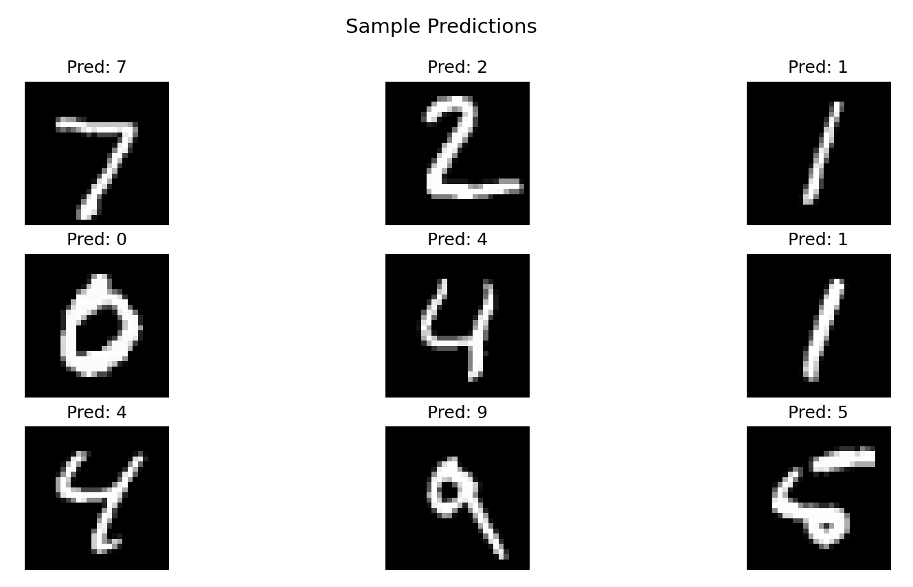
Visualize Sample Predictions
 1
 2
 3
 4
 5
 6
 7
 8
 9
10
11
12
13
14
15
16
17
18
19
20
21
22
23
24
25
26
|
import numpy as np

# Get some test images
data_iter = iter(test_loader)
images, labels = next(data_iter)
images, labels = images.to(device), labels.to(device)

# Get predictions
with torch.no_grad():
    outputs = model(images)
    _, predicted = torch.max(outputs, 1)

# Convert images to NumPy for visualization
images = images.cpu().numpy()

# Plot the images with their predicted labels
fig, axes = plt.subplots(3, 3, figsize=(8, 8))
fig.suptitle("Sample Predictions", fontsize=14)

for i, ax in enumerate(axes.flat):
    img = np.squeeze(images[i])  # Remove unnecessary dimensions
    ax.imshow(img, cmap='gray')
    ax.set_title(f"Pred: {predicted[i].item()}")
    ax.axis('off')

plt.show()
|
显示的结果
图像处理
图像裁剪代码
 1
 2
 3
 4
 5
 6
 7
 8
 9
10
11
12
13
14
15
16
17
18
19
20
21
22
|
from PIL import Image
from torchvision import transforms
from IPython.display import display
# 定义剪裁操作
center_crop_oper = transforms.CenterCrop((60,70))
random_crop_oper = transforms.RandomCrop((80,80))
five_crop_oper = transforms.FiveCrop((60,70))

# 原图
orig_img = Image.open('1.jpg')
display(orig_img)

# 中心剪裁
img1 = center_crop_oper(orig_img)
display(img1)
# 随机剪裁
img2 = random_crop_oper(orig_img)
display(img2)
# 四角和中心剪裁
imgs = five_crop_oper(orig_img)
for img in imgs:
    display(img)
|
结果

图像翻转
 1
 2
 3
 4
 5
 6
 7
 8
 9
10
11
12
13
14
15
16
17
|
from PIL import Image
from torchvision import transforms

# 定义翻转操作
h_flip_oper = transforms.RandomHorizontalFlip(p=1)
v_flip_oper = transforms.RandomVerticalFlip(p=1)

# 原图
orig_img = Image.open('1.jpg')
display(orig_img)

# 水平翻转
img1 = h_flip_oper(orig_img)
display(img1)
# 垂直翻转
img2 = v_flip_oper(orig_img)
display(img2)
|
像素取平均值
 1
 2
 3
 4
 5
 6
 7
 8
 9
10
11
12
13
14
15
16
17
18
|
from PIL import Image
from torchvision import transforms

# Ensure the image is RGB (remove alpha if necessary)
orig_img = Image.open('1.jpg').convert("RGB")

# Define normalization operation (RGB: 3 channels)
norm_oper = transforms.Normalize((0.5, 0.5, 0.5), (0.5, 0.5, 0.5))

# Convert image to tensor
img_tensor = transforms.ToTensor()(orig_img)

# Normalize
tensor_norm = norm_oper(img_tensor)

# Convert back to image
img_norm = transforms.ToPILImage()(tensor_norm)
img_norm.show()
|
Torchvision 的常用功能
torchvision.models 模块包括了一些唱功模型
基于已有的模型,做微调
- Load Pretrained Model (ResNet-18)
- Modify Last Layer for Custom Classes
- Freeze Other Layers to Use Pretrained Weights
- Train Only the New Layer (fc)
- Evaluate on Validation Set
- Save & Load Model
- Visualize Predictions
微调代码
 1
 2
 3
 4
 5
 6
 7
 8
 9
10
11
12
13
14
15
|
import torch
import torchvision.transforms as transforms
from torchvision import models
from PIL import Image

# Load ResNet18 pretrained model
model = models.resnet18(pretrained=True)

# Modify the last layer for 2 classes (e.g., Cat vs Dog)
model.fc = torch.nn.Linear(model.fc.in_features, 2)

# Move model to GPU if available
device = torch.device("cuda" if torch.cuda.is_available() else "cpu")
model.to(device)
model.eval()  # Set to evaluation mode
|
Load and Preprocess a Single Image
 1
 2
 3
 4
 5
 6
 7
 8
 9
10
11
12
13
14
15
|
from PIL import Image
import matplotlib.pyplot as plt
# Load an image
image_path = "xx.png"  # Replace with your image path
image = Image.open(image_path).convert("RGB")

# Define transformation (resize to 224x224 for ResNet)
transform = transforms.Compose([
    transforms.Resize((224, 224)),
    transforms.ToTensor(),
    transforms.Normalize([0.5, 0.5, 0.5], [0.5, 0.5, 0.5])  # Normalize to [-1, 1]
])

# Apply transformations
image = transform(image).unsqueeze(0).to(device)  # Add batch dimension
|
Perform Inference
1
2
3
4
5
6
7
|
# Get prediction
with torch.no_grad():
    output = model(image)

# Get predicted class
_, predicted = torch.max(output, 1)
print(f"Predicted class: {predicted.item()}")
|
卷积
工作原理
- 将大的 tensor 跟小 tensor 的卷积做计算
- 卷积的初始值是随机产生的
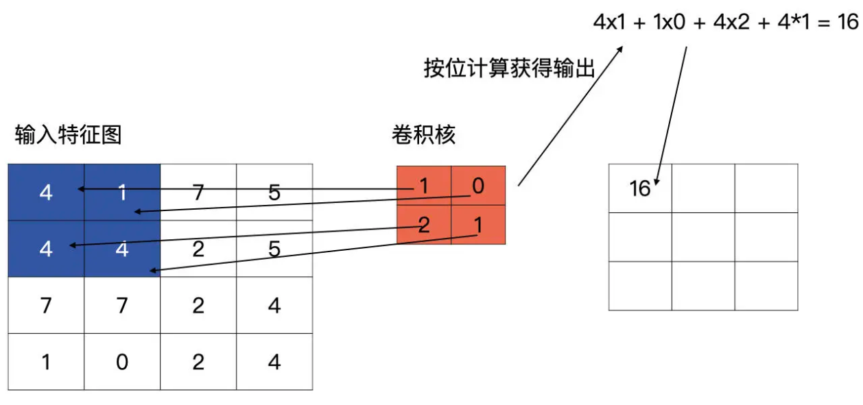
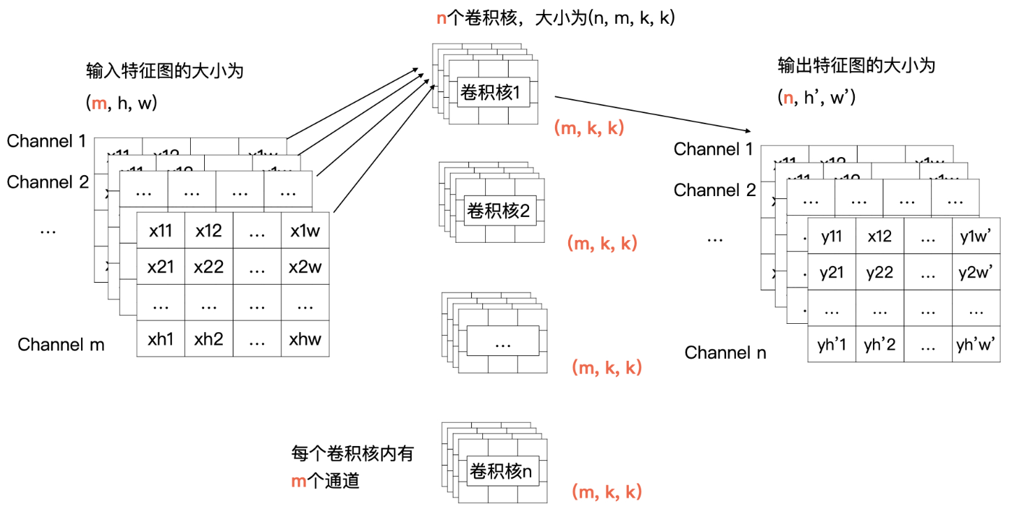
标准的卷积
- 每一个通道与卷积核中对应通道的数据做计算
- 输入特征图中第 i 个特征图与卷积核中的第 i 个通道的数据进行卷积
- 最后会产生 m 个特征图,将这 m 个特征图求和,就是最终结果
- channel 1、2、3 跟卷积1 做计算,生产结果特征 1
- n 个特征做求和就是最终特征
Padding
- 宽度高度不一致时,可以补 0
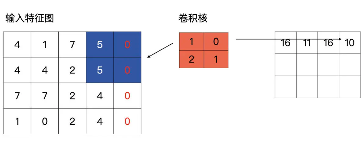
一段卷积的例子
 1
 2
 3
 4
 5
 6
 7
 8
 9
10
11
12
13
14
15
16
17
|
import torch
import torch.nn as nn

input_feat = torch.tensor([[4, 1, 7, 5], [4, 4, 2, 5], [7, 7, 2, 4], [1, 0, 2, 4]], dtype=torch.float32).unsqueeze(0).unsqueeze(0)
print(input_feat)
print(input_feat.shape)


# conv2d = nn.Conv2d(1, 1, (2, 2), stride=1, padding='same', bias=True)
conv2d = nn.Conv2d(1, 1, (2, 2), stride=2, padding=0, bias=True)
# 默认情况随机初始化参数
print(conv2d.weight)
print(conv2d.bias)

output = conv2d(input_feat)
print(output)
|
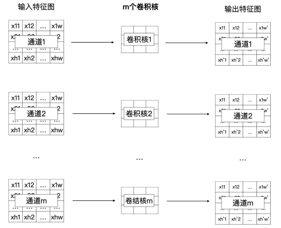
Depthwise(DW)卷积
- 减少计算量,在移动设备上也可以计算
- DW 卷积就是有 m 个卷积核的卷积,每个卷积核中的通道数为 1
- 这 m 个卷积核分别与输入特征图对应的通道数据做卷积运算
- 所以 DW 卷积的输出是有 m 个通道的特征图
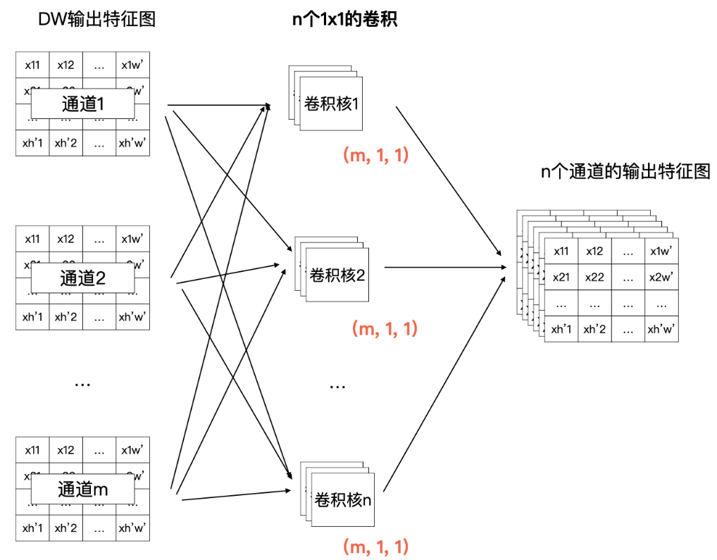
Pointwise(PW)卷积
- 也是一个 n * m 的计算矩阵
- 但是他是根据 DW 的输出来计算的,所以总体的计算量要小很多
深度可分离卷积的计算量大约为普通卷积计算量的
$\dfrac{1}{k^2}$
例子
 1
 2
 3
 4
 5
 6
 7
 8
 9
10
11
12
13
14
15
16
17
18
19
20
21
22
23
24
|
import torch
import torch.nn as nn

# 生成一个三通道的5x5特征图
x = torch.rand((3, 5, 5)).unsqueeze(0)
print(x.shape)
# 输出:
torch.Size([1, 3, 5, 5])
# 请注意DW中,输入特征通道数与输出通道数是一样的
in_channels_dw = x.shape[1]
out_channels_dw = x.shape[1]
# 一般来讲DW卷积的kernel size为3
kernel_size = 3
stride = 1
# DW卷积groups参数与输入通道数一样
dw = nn.Conv2d(in_channels_dw, out_channels_dw, kernel_size, stride, groups=in_channels_dw)

# PW 卷积
in_channels_pw = out_channels_dw
out_channels_pw = 4
kernel_size_pw = 1
pw = nn.Conv2d(in_channels_pw, out_channels_pw, kernel_size_pw, stride)
out = pw(dw(x))
print(out.shape)
|
空洞卷积
- 用来处理图像分割任务
- 感受野 会更大
对比一下普通卷积
损失函数
一个深度学习项目包括了
- 模型的设计
- 损失函数的设计
- 梯度更新的方法
- 模型的保存与加载
- 模型的训练过程等
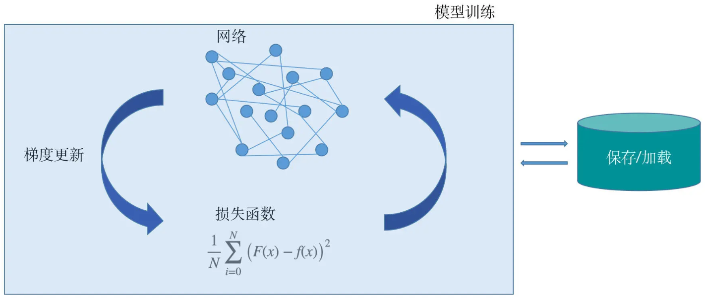
损失函数(loss fuction)
- 损失函数越小,拟合函数对于真实情况的拟合效果就越好
- 把集合所有的点对应的拟合误差做平均,就会得到如下公式
- 损失函数是单个样本点的误差,代价函数是所有样本点的误差
- $\dfrac{1}{N}\sum_{i=0}^{N}(F(x) - f(x))^2$
0-1 损失函数
$$
L(F(x), f(x)) =
\begin{cases}
0 & \text{if } F(x) = f(x)
1 & \text{if } F(x) \neq f(x)
\end{cases}
$$
Mean Squared Error (MSE),均方误差
$$
MSE = \frac{\sum_{i=1}^{n} (s_i - y_i^p)^2}{n}
$$
Mean Absolute Error (MAE),平均绝对误差损失函数
$$
MAE = \frac{\sum_{i=1}^{n} |y_i - y_i^p|}{n}
$$
信息熵的公式化可以表示为
$$
H_{\mathcal{S}} = - \sum_{i} p(x_i) \log p(x_i)
$$
交叉熵损失函数
- p(x)表示真实概率分布
- q(x) 表示预测概率分布。这个函数就是交叉熵损失函数(Cross entropy loss)
- 这个公式同时衡量了真实概率分布和预测概率分布两方面
- 所以,这个函数实际上就是通过衡量并不断去尝试缩小两个概率分布的误差,使预测的概率分布尽可能达到真实概率分布
$$
-\sum_{i=1}^{n} p(x_i) \log q(x_i)
$$
softmax 损失函数
$$
S_j = \frac{e^{a_j}}{\sum_{k=1}^{T} e^{a_k}}
$$
Weighted Log Probability Sum
- 它是交叉熵损失函数的一个特例
$$
\sum_{i=1}^{n} p(x_i) \log (S_i)
$$
对于模型来说
- 损失函数就是一个衡量其效果表现的尺子
- 有了这把尺子,模型就知道了自己在学习过程中是否有偏差,以及偏差到底有多大
计算梯度
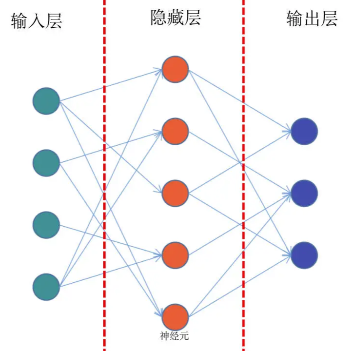
前馈网络
- 从输入层、隐藏层、再到输出层
导数
- 当函数值增量Δy 与变量 x 的增量Δx 的比值,在Δx 趋近于 0 时
- 如果极限 a 存在,我们就称 a 为函数 F(x) 在 x 处的导数
- Δx 一定要趋近于 0,而且极限 a 是要存在的
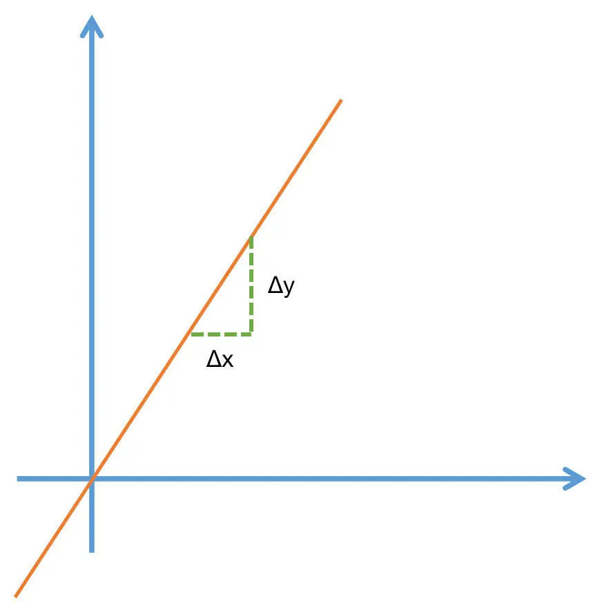
$$
f’(x_0) = \lim_{\Delta x \to 0} \frac{\Delta y}{\Delta x} = \lim_{\Delta x \to 0} \frac{f(x_0 + \Delta x) - f(x_0)}{\Delta x}
$$
偏导数
- 偏导数其实就是保持一个变量变化,而所有其他变量恒定不变的求导过程
$$
\frac{\partial}{\partial x_j} f(x_0, x_1, \dots, x_n) = \lim_{\Delta x \to 0} \frac{\Delta y}{\Delta x} = \lim_{\Delta x \to 0} \frac{f(x_0, \dots, x_j + \Delta x, \dots, x_n) - f(x_0, \dots, x_j, \dots, x_n)}{\Delta x}
$$
梯度
- 梯度向量的方向即为函数值增长最快的方向
- 模型就是通过不断地减小损失函数值的方式来进行学习的
- 让损失函数最小化,通常就要采用梯度下降的方式
- 每一次给模型的权重进行更新的时候,都要按照梯度的反方向进行
- 模型通过梯度下降的方式,在梯度方向的反方向上不断减小损失函数值,从而进行学习
$$
\nabla f(x) = \left[ \frac{\partial f}{\partial x_1}, \frac{\partial f}{\partial x_2}, \dots, \frac{\partial f}{\partial x_i} \right]
$$
链式法则
- 两个函数组合起来的复合函数,导数等于里面函数代入外函数值的导数,乘以里面函数之导数
反向传播
- 前向传播:数据从输入层经过隐藏层最后输出,其过程和之前讲过的前馈网络基本一致。
- 计算误差并传播:计算模型输出结果和真实结果之间的误差,并将这种误差通过某种方式反向传播,即从输出层向隐藏层传递并最后到达输入层
- 迭代:在反向传播的过程中,根据误差不断地调整模型的参数值,并不断地迭代前面两个步骤,直到达到模型结束训练的条件
构建网络
自定义 nn.Module 网络
 1
 2
 3
 4
 5
 6
 7
 8
 9
10
11
12
13
14
15
16
17
18
19
20
21
22
23
24
25
26
27
28
29
30
|
import torch
import torch.nn as nn
import torch.optim as optim
import torchvision
import torchvision.transforms as transforms
import matplotlib.pyplot as plt
import torch.nn.functional as F

# ✅ 1. 定义一个简单的神经网络(MLP)
class SimpleNN(nn.Module):
    def __init__(self, input_size, hidden_size, output_size):
        super(SimpleNN, self).__init__()
        self.fc1 = nn.Linear(input_size, hidden_size)  # 输入层 → 隐藏层
        self.relu = nn.ReLU()  # 激活函数
        self.fc2 = nn.Linear(hidden_size, output_size)  # 隐藏层 → 输出层

    def forward(self, x):
        x = self.fc1(x)
        x = self.relu(x)
        x = self.fc2(x)
        return x

# ✅ 2. 创建模型
input_size = 28 * 28  # MNIST 图像大小(28x28)
hidden_size = 128  # 隐藏层神经元数量
output_size = 10  # MNIST 10 个类别(0~9)
model = SimpleNN(input_size, hidden_size, output_size)

# ✅ 3. 查看模型结构
print(model)
|
训练模型
 1
 2
 3
 4
 5
 6
 7
 8
 9
10
11
12
13
14
15
16
17
18
19
20
21
22
|
# ✅ 1. 加载 MNIST 数据集
transform = transforms.Compose([transforms.ToTensor(), transforms.Normalize((0.5,), (0.5,))])
trainset = torchvision.datasets.MNIST(root="./data", train=True, download=True, transform=transform)
trainloader = torch.utils.data.DataLoader(trainset, batch_size=64, shuffle=True)

# ✅ 2. 定义损失函数和优化器
criterion = nn.CrossEntropyLoss()
optimizer = optim.Adam(model.parameters(), lr=0.001)

# ✅ 3. 训练模型
epochs = 5
for epoch in range(epochs):
    for images, labels in trainloader:
        images = images.view(-1, 28*28)  # 展平图像
        optimizer.zero_grad()  # 清空梯度
        outputs = model(images)  # 前向传播
        loss = criterion(outputs, labels)  # 计算损失
        loss.backward()  # 反向传播
        optimizer.step()  # 更新参数
    print(f"Epoch {epoch+1}/{epochs}, Loss: {loss.item():.4f}")

print("训练完成!")
|
微调 ResNet18
 1
 2
 3
 4
 5
 6
 7
 8
 9
10
11
12
13
14
15
16
17
18
19
20
21
22
23
24
25
26
27
28
29
30
31
32
33
34
|
from torchvision import models

# ✅ 1. 加载预训练模型
pretrained_model = models.resnet18(pretrained=True)

# ✅ 2. 替换 ResNet18 的最后一层(适配 MNIST 10 类)
pretrained_model.fc = nn.Linear(512, 10)  # ResNet18 的全连接层输入是 512

# ✅ 3. 冻结除最后一层以外的所有参数
for param in pretrained_model.parameters():
    param.requires_grad = False  # 冻结所有层
pretrained_model.fc.requires_grad = True  # 只训练最后一层

# ✅ 4. 迁移到 GPU
device = torch.device("cuda" if torch.cuda.is_available() else "cpu")
pretrained_model = pretrained_model.to(device)

# ✅ 5. 定义优化器和损失函数
optimizer = optim.Adam(pretrained_model.fc.parameters(), lr=0.001)
criterion = nn.CrossEntropyLoss()

# ✅ 6. 训练微调模型
epochs = 3
for epoch in range(epochs):
    for images, labels in trainloader:
        images, labels = images.to(device), labels.to(device)
        optimizer.zero_grad()
        outputs = pretrained_model(images)
        loss = criterion(outputs, labels)
        loss.backward()
        optimizer.step()
    print(f"Epoch {epoch+1}/{epochs}, Loss: {loss.item():.4f}")

print("微调完成!")
|
优化方法
优化方法
- 目的就是找到能够使得 f(x) 的值达到最小值对应的权重
- 优化过程就是找到一个状态,这个状态能够让模型的损失函数最小,而这个状态就是模型的权重
- 梯度向量的方向即为函数值增长最快的方向,梯度的反方向则是函数减小最快的方向
梯度下降 vs 贪心
| 特性 |
梯度下降 |
贪心算法 |
| 应用领域 |
连续优化问题(如神经网络训练) |
离散/组合优化问题(如最短路径、背包问题) |
| 决策依据 |
利用局部导数(梯度)信息 |
局部最优选择(直接选择当前最优的选项) |
| 更新方式 |
迭代更新参数,逐步逼近最优 |
一步步构造解,决策一经做出便不再调整 |
| 全局最优性 |
在凸问题下可达全局最优,非凸问题可能陷入局部最优 |
局部最优不一定能构造出全局最优解 |
| 依赖条件 |
目标函数必须可微,以计算梯度 |
依赖问题的局部评估准则,无需可微性 |
常见的梯度下降方法
- 批量梯度下降法(Batch Gradient Descent,BGD)
- 随机梯度下降(Stochastic Gradient Descent,SGD)
- 随机梯度下降方法选择了用损失很小的一部分精确度和增加一定数量的迭代次数为代价,换取了最终总体的优化效率的提高
- 小批量梯度下降(Mini-Batch Gradient Descent, MBGD)
为了得到最小的损失函数,我们要用梯度下降的方法使其达到最小值
要点:模型之所以使用梯度下降,其实是通过优化方法不断的去修正模型和真实数据的拟合差距

范围
机器学习开发的几个步骤
- 数据处理:主要包括数据清理、数据预处理、数据增强等。总之,就是构建让模型使用的训练集与验证集
- 模型训练:确定网络结构,确定损失函数与设置优化方法
- 模型评估:使用各种评估指标来评估模型的好坏
可视化工具
安装
1
|
pip install tensorboard
|
测试
 1
 2
 3
 4
 5
 6
 7
 8
 9
10
11
12
13
14
15
16
17
18
19
20
21
|
from torch.utils.tensorboard import SummaryWriter
# PyTorch 1.8之前的版本请使用:
# from tensorboardX import SummaryWriter
import numpy as np

# 创建一个SummaryWriter的实例
writer = SummaryWriter()

for n_iter in range(100):
    writer.add_scalar('Loss/train', np.random.random(), n_iter)
    writer.add_scalar('Loss/test', np.random.random(), n_iter)
    writer.add_scalar('Accuracy/train', np.random.random(), n_iter)
    writer.add_scalar('Accuracy/test', np.random.random(), n_iter)


img = np.zeros((3, 100, 100))
img[0] = np.arange(0, 10000).reshape(100, 100) / 10000
img[1] = 1 - np.arange(0, 10000).reshape(100, 100) / 10000

writer.add_image('my_image', img, 0)
writer.close()
|
在当前目录下会生成 run,之后执行
1
|
tensorboard --logdir=runs
|

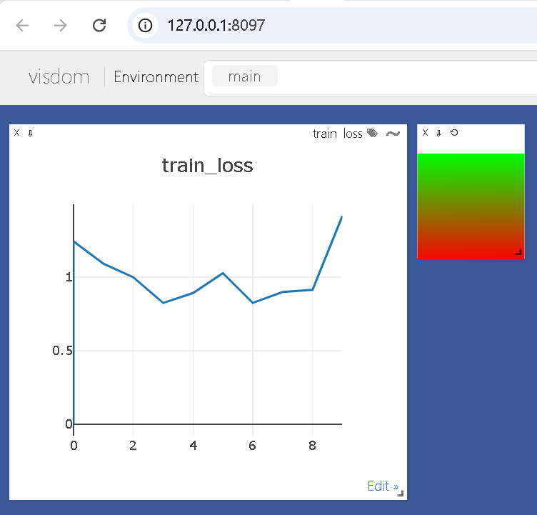
Visdom
运行
1
|
python -m visdom.server
|
测试代码
 1
 2
 3
 4
 5
 6
 7
 8
 9
10
11
12
13
14
15
16
17
18
19
20
21
|
from visdom import Visdom
import numpy as np
import time

# 将窗口类实例化
viz = Visdom()
# 创建窗口并初始化
viz.line([0.], [0], win='train_loss', opts=dict(title='train_loss'))

for n_iter in range(10):
    # 随机获取loss值
    loss = 0.2 * np.random.randn() + 1
    # 更新窗口图像
    viz.line([loss], [n_iter], win='train_loss', update='append')
    time.sleep(0.5)

img = np.zeros((3, 100, 100))
img[0] = np.arange(0, 10000).reshape(100, 100) / 10000
img[1] = 1 - np.arange(0, 10000).reshape(100, 100) / 10000
# 可视化图像
viz.image(img)
|
实时更新状态
分布式训练
测试
 1
 2
 3
 4
 5
 6
 7
 8
 9
10
11
12
|
import torch
data = torch.ones((3, 3))
print(data.device)
# Get: cpu

# 获得device
device = torch.device("cuda: 0")

# 将data推到gpu上
data_gpu = data.to(device)
print(data_gpu.device)
# Get: cuda:0
|
单机并行化
1
|
torch.nn.DataParallel(module, device_ids=None, output_device=None, dim=0)
|
多机多卡
DistributedDataParallel
- 实现多机多卡的关键 API
- 既可用于单机多卡也可用于多机多卡
例子
 1
 2
 3
 4
 5
 6
 7
 8
 9
10
11
12
13
14
15
16
17
18
19
20
21
22
23
24
25
26
27
28
29
30
31
32
33
34
35
36
37
38
39
40
41
42
43
44
45
46
47
48
|
import os
import torch
import torch.nn as nn
import torch.optim as optim
import torch.distributed as dist
import torch.multiprocessing as mp
from torch.nn.parallel import DistributedDataParallel as DDP

def train(rank, world_size, master_ip):
    """ Initialize distributed training """
    os.environ["MASTER_ADDR"] = master_ip
    os.environ["MASTER_PORT"] = "29500"  # Standard PyTorch port

    # Initialize the process group (NCCL for GPU communication)
    dist.init_process_group("nccl", rank=rank, world_size=world_size)

    # Assign correct GPU to each rank
    device = torch.device(f"cuda:{rank % torch.cuda.device_count()}")

    # Create model and move it to the assigned GPU
    model = nn.Linear(10, 1).to(device)
    model = DDP(model, device_ids=[device])

    # Define loss function and optimizer
    criterion = nn.MSELoss()
    optimizer = optim.SGD(model.parameters(), lr=0.01)

    # Dummy data
    x = torch.randn(5, 10).to(device)
    y = torch.randn(5, 1).to(device)

    for epoch in range(5):
        optimizer.zero_grad()
        output = model(x)
        loss = criterion(output, y)
        loss.backward()
        optimizer.step()
        print(f"Rank {rank}, Epoch {epoch}, Loss: {loss.item()}")

    # Cleanup
    dist.destroy_process_group()

if __name__ == "__main__":
    world_size = 2  # Number of machines (Master + Worker)
    rank = int(os.environ["RANK"])  # Get rank from environment variables
    master_ip = os.environ["MASTER_IP"]  # Get master node IP

    train(rank, world_size, master_ip)
|
两台机器的启动参数
 1
 2
 3
 4
 5
 6
 7
 8
 9
10
11
|
export MASTER_IP=192.168.1.10
export RANK=0
export WORLD_SIZE=2
export CUDA_VISIBLE_DEVICES=0
python train.py

export MASTER_IP=192.168.1.10  # Must point to the Master Node
export RANK=1
export WORLD_SIZE=2
export CUDA_VISIBLE_DEVICES=0
python train.py
|
参考